This page explains the mathematical techniques and software algorithms I use to manipulate bell sounds for various purposes. The results in the next section, showing how the partial frequencies of bells can be altered and the effect on their sound, will be of interest to anyone acquainted with bell acoustics. The techniques include:
- Sharpening or flattening a bell sound as a whole
- Changing the frequency of an individual partial
- Stretching or shrinking all the upper partials together to give the effect of thinner or thicker bells.
Though the algorithms may not look simple (especially the technique used to change the upper partials) they are very fast. Stretching or shrinking upper partials in a bell sound, or changing multiple partials below the nominal, using a python program and the numpy package takes a few lines of code and runs in a fraction of a second.
In the past, I have attempted to create bell sounds with particular characteristics (e.g. a set of partial frequencies) from the partial frequencies, amplitudes, attack and decay times. The results are not very realistic, both because bell sounds contain a large number of partials, and because clappering and the acoustics of the bellchamber play an important role. On the other hand, recordings of real bells adjusted to give the partials of interest give a very realistic result.
In the next section, there are a set of bell sounds produced using the techniques described. The rest of the article give the detail of the techniques.
Sound samples
Here are a set of bell sounds produced using these techniques. The original sound is that of a Taylor bell weighing around 5 cwt. The partial frequencies of the various sounds are as follows:
| File | Hum | cents | Prime | cents | Tierce | cents | Quint | cents | Nominal | S’quint | cents | Oct Nom | cents |
|---|---|---|---|---|---|---|---|---|---|---|---|---|---|
| original | 345 | -2399.4 | 688 | -1204.4 | 823 | -894.2 | 1025.5 | -513.4 | 1379.5 | 2042 | 679.0 | 2776.5 | 1210.9 |
| semitone | 365.5 | -2399.4 | 728.5 | -1205.3 | 872 | -894.1 | 1086.5 | -513.3 | 1461.5 | 2163 | 678.7 | 2941.5 | 1210.9 |
| old style | 370 | -2278.3 | 640 | -1329.6 | 829 | -881.6 | 1025.5 | -513.4 | 1379.5 | 2042 | 679.0 | 2776.5 | 1210.9 |
| oct. nom. 1180 | 345 | -2399.4 | 688 | -1204.4 | 823 | -894.2 | 1025.5 | -513.4 | 1379.5 | 2021.5 | 661.5 | 2727 | 1179.8 |
| oct. nom. 1280 | 345 | -2399.4 | 688 | -1204.4 | 823 | -894.2 | 1025.5 | -513.4 | 1379.5 | 2088 | 717.6 | 2889.5 | 1280.0 |
It should be apparent from these sounds that the fine details of the original recording such as the sound of the clapper bouncing on the bell, and the acoustics of the bellchamber, are preserved by the manipulation.
Sound file formats
All these techniques are intended for application to sound files formatted as PCM – for example, to windows .wav files. Sound files for this format are uncompressed, and comprise a time-series of digital values of the analogue waveform. The number of samples per second is known as the sampling rate. A common rate (used for example for CD-format music) is 44,100 samples per second. The techniques are independent of the sampling rate, but with an important caveat.
A theorem known as the Sampling Theorem states that the maximum frequency that can be represented with a sampling rate s is half that rate, i.e. s/2. This frequency is known as the Nyquist frequency. So with a sampling rate of 44,100 samples per second, the maximum practical frequency in the sound is 22,050 Hz (cycles per second). Partial frequencies in bells sounds are found up to 10,000 Hz, or 15,000 Hz in very small bells. How high the maximum frequency in a recording is depends on the quality of the recording equipment as well as the original sound.
If a bell sound is digitised at a low sampling rate, such as 8,000 samples per second, any frequencies higher than the Nyquist frequency (which in this case would be 4,000 Hz) are aliased to a frequency below the Nyquist frequency. A recording at such a low sampling rate may not sound too bad, but an attempt to apply the techniques in this article to such a sound may produce poor results.
The sampling rate is different from the number of bits per second used to represent the sound. Compressed sound formats such as mp3 and m4a can significantly reduce the number of bits needed to represent the sound, but the underlying sampling rate remains high. Sounds in these compressed formats can be expanded to PCM (e.g. a .wav file) with a sound editor such as Audacity.
Interpolation
All the techniques in this article use interpolation of values in time or frequency, so that technique is covered first. As an example, if it is desired to sharpen or flatten a bell sound, the sound can be re-sampled in the time domain to alter its length. This changes all the partial frequencies by the same ratio, so the intervals between them are unchanged, though the absolute frequencies are different.
if the original sound has a sampling rate of 44,100 samples per second then an analogue value is captured every 1/44100 of a second. if it is required to sharpen the sound by one semitone, a ratio of approximately 1.059, we need to create a new waveform by taking values from the old waveform spaced by 1.059/44100 which is approximately 1/41643 of a second. Most of the new values will lie between values in the original sound file. Interpolation allows us to calculate these intermediate values. The resulting sound file will be slightly shorter than the original one.
This plot shows the first 11 samples of an arbitrary waveform:
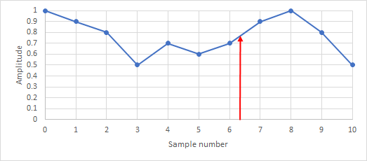
If this waveform is to be shrunk or sharpened by a semitone, then sample 6 in the new waveform needs to be the value corresponding to position 6 * 1.059 ≈ 6.35 in the original sound. This position is shown by the red arrow in the plot. An approximate value for the waveform at this point can be calculated assuming a straight line between the values for points 6 and 7 – so-called linear interpolation. If v6 is the value of sample 6 and v7 the value of sample 7, the value for position 6.35 is v6 + 0.35 * (v7 – v6). This calculation applied successively for each sample in the new waveform creates the new sound.
Linear interpolation using just the two samples either side of the desired value is a special case of interpolation techniques using more samples from the original. (Ref 1 page 105 onwards, Ref 2) Because the frequencies in bell sound recordings are typically rather less than both the sampling rate and the Nyquist frequency (half the sampling rate), practical experience has shown that linear interpolation gives musically very satisfactory results.
Linear interpolation is built into the basic operation of Wavanal. If the user selects a frequency interval of e.g. 0.5Hz, the sound is resampled prior to the fourier transform so that the frequency bins are spaced by exactly 0.5Hz in the result. Extensive testing and many years of experience have shown that this resampling produces valid results for the transform and the partial frequencies.
Sharpening or flattening a bell sound
The ‘Increase Freq.’ facility in Wavanal uses the above interpolation technique to stretch or shrink the waveform. The user can choose the amount of stretching or shrinking either by specifying the new value of a particular frequency – usually the nominal – or the change in cents required. As explained above, the stretch or shrink of the waveform flattens or sharpens the sound but leaves the intervals between all the partials unchanged.
It is likely that very large amounts of shrink and stretch will stress the algorithm because of the many interpolated points, or the many omitted samples. Shrinking or stretching by a semitone or a tone gives results that are musically very satisfactory.
Changing the frequency of an individual partial
This task is more complex because the individual partial needs to be extracted from the sound and modified. The basic steps implemented in a python program are as follows:
- fourier-transform the sound file to get its representation in frequency space
- filter this transform to extract the partial of interest from the transform
- using an inverse filter, produce a transform omitting the partial of interest
- do the inverse transforms to generate two sound files, one for the partial of interest, and one for the bell sound omitting the partial of interest
- stretch or shrink the sound of the individual partial to change its frequency as required, using the interpolation technique described above
- add the sound of the stretched or shrunk partial back to the sound.
The stretch or shrink of the soundfile for the partial of interest changes its length, which affects its attack and decay time a little. However, this seems to have no impact on the results.
The filter used is important to the success of the procedure. A simple square filter extracting or excluding frequencies in a band either side of the partial frequency produces poor results because of the Gibbs phenomenon, giving ringing in the waveform after the inverse transform because of the sharp filter edges. Instead, a Gaussian function is used as the filter centred on the partial frequency. This filter shape minimises the ringing due to Gibbs, an example of the Hardy uncertainty principle which says that no function is better localised together with its fourier transform that the Gausssian. (Ref 1 page 607, ref 3) The parameters of the Gaussian were chosen to give appropriate separation between adjacent partial frequencies.
Here is an example of a gaussian filter centred on 800 Hz. The actual filter used extends up to the Nyquist frequency (e.g. 22,050 Hz) but all the higher values are zero:
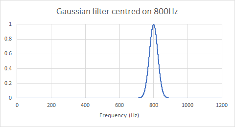
The inverse filter used to exclude this frequency from the transform is just 1.0 – filter_values.
To avoid doing repeated transforms and inverse transforms to adjust multiple partials, the python program loops across all the partials to be adjusted, extracting each one and adding the notch filter for each to the filter to be applied to the remaining sound, before applying this filter and doing the inverse transform.
Stretching or shrinking the upper partials
In principle, changing the upper rim partials to create the effect of a thinner or thicker bell could use the technique explained in the previous section, applied to multiple partials – up to seven in a typical bell sound. However this approach has two disadvantages:
- The current and desired frequencies of seven or more partials would need to be specified
- Modifying this many different frequencies in the bell sound might have poor results.
Instead, the technique used takes advantage of the relationship between all the upper rim partials, as shown in the following plot:
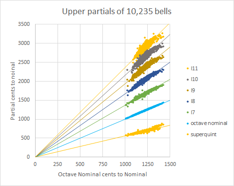
The cents of each upper rim partial to the nominal varies linearly with the cents of the octave nominal to the nominal. The solid lines in the plot are regression lines passing through the origin. So, if all the frequencies in the sound above the nominal are stretched or shrunk by an appropriate amount, the relationship between all the upper rim partials will be preserved. Taking this approach alters the frequencies of all the partials above the nominal, but the rim partials are so much more musically important than any of the others that this is not material.
The amount of shrink or stretch required can be conveniently expressed by giving the current and desired cents for the octave nominal relative to the nominal. The shrink or stretch can be implemented by interpolating from a Fourier transform of the original bell sound, and doing an inverse transform on the interpolated transform. To express the procedure mathematically, some symbols need to be defined.
fn is the nominal frequency
fu is the frequency of a particular upper partial (superquint, octave nominal, I7 etc.)
cu is the cents of this partial relative to the nominal
fon is the frequency of the octave nominal
con is the cents of the octave nominal to the nominal
K is the constant 1200.0 / loge(2) ≈ 1731.234 to seven significant figures, so that, for example, con = K * loge(fon / fn)
Values with primes (e.g. fu‘) are the values after the shrink or stretch of the upper partials.
To do the required calculation, for each shrunk or stretched upper partial frequency fu‘ we need to know at what point fu to look in the original transform for the required value. If we assume the linear relationship between cu and con, and that the line passes through the origin for all upper rim partials, then cu = ku * con and cu‘ = ku * con‘ where ku is a constant for upper partial u. Re-arranging these two formulas and eliminating ku gives:
cu‘ / con‘ = cu / con
i.e. K * loge(fu / fn) = K * loge(fu‘ / fn) * con / con‘
Eliminating K and expanding the logs gives:
loge(fu) – loge(fn) = con / con‘ * { loge(fu‘) – loge(fn) }
A final re-arrangement gives:
fu = exp{ (1 – con / con‘) * loge(fn) + con / con‘ * loge(fu‘) } where exp represents the exponent or antilog function.
This transformation needs to be applied to every frequency in the transform above the nominal. The value (1 – con / con‘) * loge(fn) is a constant for a particular degree of stretch or shrink and can be taken out of the loop across all frequencies. The transform values are complex numbers and the interpolation calculation needs to accommodate that. For a real-mode Fourier transform, the index into the transform array can be calculated from the frequency by multiplying by transform_length / sample_rate / 2.0.
The procedure for stretching or shrinking the upper partials, while leaving the nominal and lower partials unchanged, is as follows:
- note the nominal frequency, the current octave nominal cents and the desired octave nominal cents
- do a fourier transform of the original sound
- copy this transform unchanged to the new transform up to the nominal frequency
- above the nominal frequency, use the formula above to interpolate transform values from the original to the new transform
- carry out the inverse transform.
References
References are given to Numerical Recipes. This is now an old book, and is criticised, but it still gives a good introduction to the topics of interest.
- Press W H, Teukolsky S A, Vettering W T, Flannery B P, Numerical Recipes in C, 2nd Edition, Cambridge University Press, 2002
- Wikipedia article on Interpolation
- Wikipedia article on the Gibbs phenomenon